Forecasting, making predictions about the future, plays a key role in the decision-making process of any company that wants to maintain a successful business. This is due to the fact that success tomorrow is determined by the decisions made today, which are based on forecasts. Hence good forecasts are crucial, for example, for predicting sales to better plan inventory, forecasting economic activity to inform business development decisions, or even predicting the movement of people across an organization to improve personnel planning.

In this post, we demonstrate how to leverage multiple historical time series in conjunction with Recurrent Neural Networks (RNN), specifically Long Short-Term Memory (LSTM) networks [1], to make predictions about the future. Furthermore, we use a method based on DeepLIFT [4][5] to interpret the results.

We choose this modeling approach because it delivers state-of-the-art performance in settings where traditional methods are not suitable. In particular, when the time series data is complex, meaning trends and seasonal patterns change over time, deep learning methods like LSTM networks are a viable alternative to more traditional methods such as ARMA (Auto-Regressive Moving Average) [2]. Originally developed for Natural Language Processing (NLP) tasks, LSTM models have made their way into the time series forecasting domain because, as with text, time series data occurs in sequence and temporal relationships between different parts of the sequence matter for determining a prediction outcome.

Additionally, we want to shed some light on the trained neural network by finding the important features that contribute most to the predictions.

The example we use is to forecast the future price of Bitcoin based on historical times series of the price itself, as well as other features such as volume and date-derived features. We choose this data because it exemplifies the dynamically changing, behavioral aspects of decisions made by individual investors when they decide to buy or sell the asset. These aspects do also appear in other forecasting problems such as those mentioned in the introduction. This post is written for educational purposes only and you should not see it as investment advice.

Data Exploration & Preparation

The dataset consists of daily prices including Open, High, Low, Close (all quoted in US Dollar), as well as Volume (daily traded volume in US Dollar) starting in July 2016 to July 2021.

The following chart shows the time series of the daily closing price (Fig. 1). You can already see that the time series is characterized by frequent spikes, troughs, as well as changing (local) trends.
 

Time Series Stationarity

Traditional statistical forecasting techniques require the data to be stationary, i.e., having constant mean, standard deviation, and autocorrelation. If, however, the conditions for stationarity are not achieved, forecasting techniques, like ARMA, cannot model the dependence structure of the data over time and therefore other techniques have to be used.

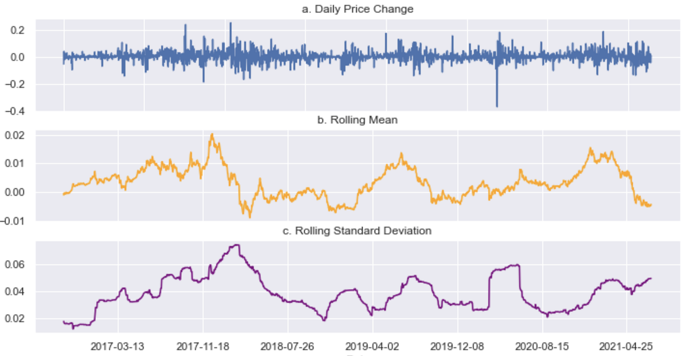
Let’s take a closer look at our example and do some visual checks. Simply from eyeballing the above price time series (Fig. 1), you can see that it is not stationary as the mean changes over time. Typical for time series problems, the next step would be to transform the time series to try to make it stationary. We take the first order percentage difference of the price levels to obtain daily price changes. Additionally, we calculate the rolling mean as well as the rolling standard deviation of the daily price changes over time. In Figure 2, you can see that neither the mean nor the standard deviation of daily price changes are constant over time, hence the time series is not stationary.
 

Feature Generation and Preparation

We derive two more features from the dataset, including the percentage difference between High and Low as a measure for intra-day price movement and the percentage difference between next-day Open and Close as a measure for overnight price movement. Additionally, we derive three features from the date column including day of week, month of year, and quarter of year to help predict our target feature, the closing price (Close).

Given that our financial time series data is relatively clean and structured, we don’t have to spend much time cleaning and preparing the data. The preparation steps include splitting our dataset into training and test sets as well as rescaling all features to a common scale between 0 and 1 which helps preventing model overfit when the features are in different scales. Normally, we would keep a hold-out dataset for the evaluation of the model at the end of the analysis, but observing the model’s performance on the test dataset shall suffice in our case.

Multivariate Time Series Forecasting

Next, we dedicate ourselves to building a time series forecasting model, that can take multiple variables (with their respective histories) as inputs, to predict the future price.

Objective

Before we dive into the modeling aspect, it is essential to identify an objective (or cost) function that is aligned with the business goal to ensure the model can actually help achieve the desired business outcome. The goal is to create a forecasting model that predicts the price as closely as possible while prioritizing more permanent price movements (e.g., weekly trends) over smaller, more variable intra-week movements.

We make the following considerations:

• We choose Mean-Squared-Error (MSE) as our primary cost function given that our dataset is of high quality, i.e., there are no outliers as a result of data errors that could otherwise result in model overfit using this error metric.
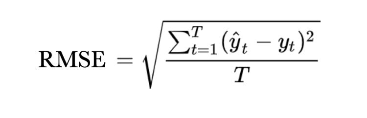
• We actually pick Root-MSE (RMSE), see Fig. 3, over MSE for the simple reason of better interpretability since RMSE has the same unit as the predicted variable.
• In other scenarios, such as predicting sales, the data can potentially be erroneous, e.g. if holidays are not accounted for. The model would falsely predict low sales and the resulting large error would wrongfully be penalized during training.
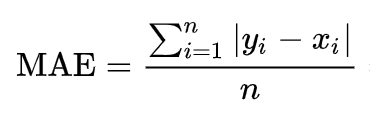
• Given the presence of some large but rare price swings in our data, RMSE can potentially lead to model overfit. Furthermore, we’re more interested in predicting the general trend rather than short-term movements of the time series. Hence, we opt to include Mean-Absolute-Error (MAE), see Fig. 4, as an additional performance measure because it is more forgiving to outliers than RMSE.
   

We aim to minimize RMSE as well as MAE.

Recurrent Neural Networks & Long Short-Term Memory

Let’s focus on building the forecasting model. For that, we’ll quickly review Recurrent Neural Networks (RNN) as well as Long Short-term Memory (LSTM) networks.

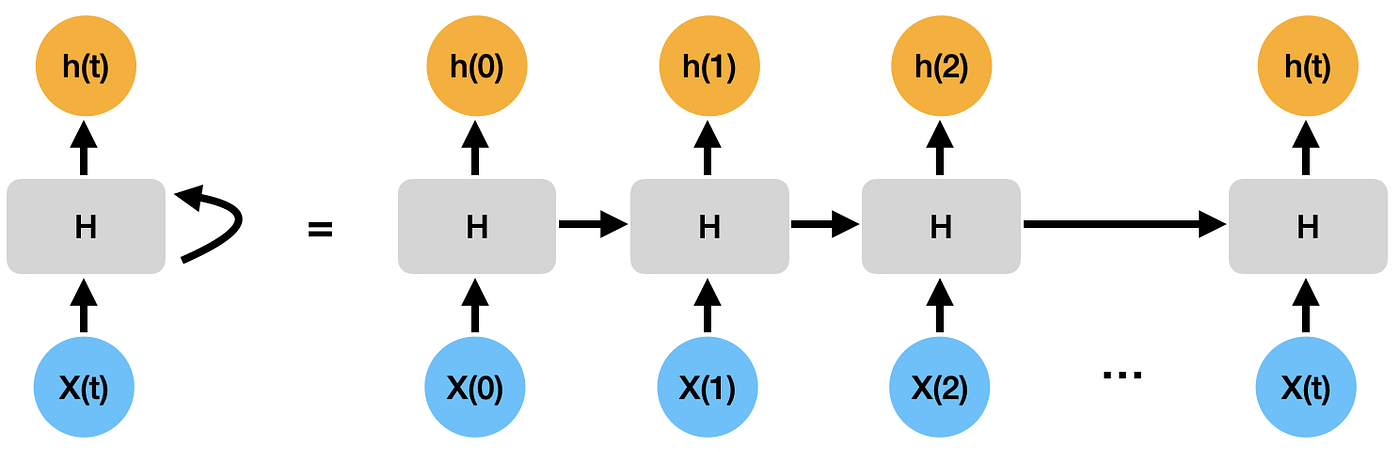
RNNs are a type of neural network architecture which is mainly used to detect patterns in sequential data such as language, or, as in our case, numerical time series. To detect the sequential patterns in the data, information is passed through the network with cycles, i.e., the information is transmitted back into the model [3]. This enables the RNN to take into account previous inputs X(t-1) in addition to the current input X(t). In Fig. 5, you can see how information, h(t), from one step of the network is passed to the next.
 

LSTMs, a special type of RNNs, were designed to handle such long range dependencies much better than standard RNNs [1][3]. Similar to RNNs, LSTMs have a chain-like structure but each repeating block, a LSTM cell, has 3 additional fully-connected layers compared to the one of the standard RNN (Fig. 6). These additional layers are also called gate layers because of their different activation (sigmoid) compared to the standard layer (tanh). As the information passes through each LSTM cell, the cell state, C(t), can be updated by adding or removing information via the gate layers. This is how the LSTM model decides whether to retain or drop information from previous time steps.
 

For more details and the exact structure of LSTMs, you can refer to [1].
 

Model Training and Evaluation

Our specific forecasting model consists of two LSTM layers followed by one fully connected layer to predict the following day’s price. We employ a dataset class to generate time series of our feature set with a sequence length of 30 days and a dataloader class to load them in batches. We train the model using the Adam optimizer and RMSE as well as MSE as loss functions (during separate runs). Furthermore, we implement early-stopping to allow the training job to finish early if there are no significant performance improvements.

Since the input data was scaled to levels between 0 and 1, we have to scale back (descale) the model’s outputs to the original scale to be able to assess the predictions against the actual price levels. The focus is not about tuning the best model, so we train with just one set of hyperparameters and consider this a baseline model. After training the model for about 10–15 epochs and descaling its outputs, the model achieves an RMSE of about 10,000 and a MAE of about 6,500 on the test dataset.

Let’s have a look at the predictions on the test data (Fig. 7). You can see that the model does relatively well with predicting the overall price development, which was our objective, for the first quarter of the test dataset. At around the middle (300–450 days), the model seems to constantly overestimate the price and it fails to predict the extreme price increase towards the end (680 days and after) which explains the large errors noted above.
 

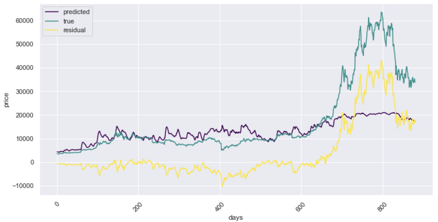
The fact that the model fails to predict several spikes and troughs of the price is indicative of missing input factors. Adding more features to the training dataset could help improve the model predictions further.

This is not considered an exhaustive analysis into the model’s prediction errors but it shall suffice for our purpose. Next, we will use this baseline model and try to explain its predictions.

Important Features

Understanding why the model makes the predictions it makes can be difficult in the case of neural networks. We use an approach that is based on the DeepLIFT algorithm [4][5] which approximates the SHAP values known from classic game theory. Basically, this approach seeks to answer the question of how much a feature contributes to a model’s predictions when it’s there (in the inputs) compared to when it’s not there (not in the inputs), thus deriving the feature’s importance. More specifically, the method decomposes the output prediction of a neural network on a specific input by backpropagating the contributions of all neurons in the network to every feature of the input. It then compares the activation of each neuron to its reference activation and assigns contribution scores (or multipliers) according to the difference. The reference input represents some default or neutral input that is chosen depending on the domain, e.g., zeros or feature averages. Once the multipliers have been computed based on a representative dataset (or background dataset), we can calculate the contributions of the input features to the model’s output based on some sample inputs and rank the features in order of their largest contributions to get their importance.

We use 900 training data samples as the background dataset and 100 test data samples on which to explain the model’s output. Since the feature importances are calculated for each input sample at each time step, we average them across all 100 input samples and plot the importances by feature as well as by time step (Fig. 8). The top 3 input features are Volume, Close Price, and the intraday High-Low Percentage Price Change. We can also see that more recent time steps, days -7 to -1, play a more significant role in making predictions compared to time steps further away, days -30 to -8, where day 0 is the time of prediction.
 

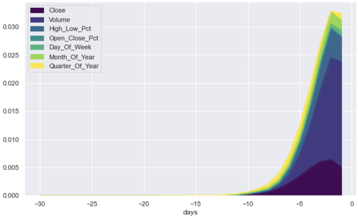
Furthermore, the insights from finding the important features can also help inform the model optimization process. For example, here, cutting the input sequence length as well as removing unimportant features would increase training and inference speed while likely not affecting the prediction performance by much.

Conclusion

In this post, we showed how to build a multivariate time series forecasting model based on LSTM networks that works well with non-stationary time series with complex patterns, i.e., in areas where conventional approaches will lack. After aligning the forecasting objective with our ‘business’ goal, we trained and evaluated the model with little data preparation required. Additionally, we found out what features (and what time steps) drive the model’s predictions using a technique based on DeepLIFT. This allows us to interpret the deep learning model and derive better decisions from it.

The Github code accompanying this blog post can be found here.

References:

[1] Hochreiter and Schmidhuber. “Long Short-term Memory”. (1997)

[2] Box and Jenkins. “Time Series Analysis, Forecasting and Control”. (1994)

[3] Schmidt. “Recurrent Neural Networks (RNNs): A gentle Introduction and Overview”. (2019)

[4] Shrikumar, Greenside, and Kundaje. “Learning Important Features Through Propagating Activation Differences”. (2017)

[5] Lundberg and Lee. “A Unified Approach to Interpreting Model Predictions”. (2017)